Linear Discriminant Analysis (LDA)

According to Bayes’ Theorem, the posterior distribution that a sample \(x\) belong to class \(l\) is given by

\[\pi (y=C_l|x) = \frac{\pi (y=C_l)\pi(x|y=C_l)}{\sum_{l=1}^C \pi(y=C_l)\pi(x|y=C_l)}\]

where \(\pi(y=C_l)\) is the prior probability of membership in class \(C_l\) and \(\pi(x|y=C_l)\) is the conditional probability of the predictors \(x\) given hat data comes from class \(C_l\).

The rule that minimizes the total probability of misclassification says to classify \(x\) into class \(C_k\) if \(\pi(y=C_k)\pi(x|y=C_k)\) has the largest value across all of the \(C\) classes.

If we assume that \(\pi(x|y=C_l)\) follows a multivariate Gaussian distribution \(\Phi(\mu_l,\Sigma)\) with a class=specific mean vector \(\mu_l\) and a common covariance matrix \(\Sigma\) we have that the log of \(\pi(y=C_k)\pi(x|y=C_k)\) is given by

\[x^T \Sigma^{-1}\mu_l - 0.5\mu_l^T \Sigma^{-1}\mu_l + \log(\pi(y=C_l))\]

which is a linear function in \(x\) that defines separating class boundaries, hence the name LDA.

LDA can be seen from two different angles. The first classify a given sample of predictor \(x\) to the class \(C_l\) with highest posterior probability \(\pi(y=C_l|x)\), where LDA minimizes the total probability of misclassification, as mentioned. The second tries to find a linear combination of the predictors that gives maximum separation between the centers of the data while at the same time minimizing the variation within each group of data.

In this post, I will express the first aspect of LDA. The second one will be showed in the next post.

LDA as a classifier

We are going to investigate LDA using the iris dataset. The data contains four continuous variables which correspond to physical measures of flowers and a categorical variable describing the flowers’ species.

head(iris)

##   Sepal.Length Sepal.Width Petal.Length Petal.Width Species
## 1          5.1         3.5          1.4         0.2  setosa
## 2          4.9         3.0          1.4         0.2  setosa
## 3          4.7         3.2          1.3         0.2  setosa
## 4          4.6         3.1          1.5         0.2  setosa
## 5          5.0         3.6          1.4         0.2  setosa
## 6          5.4         3.9          1.7         0.4  setosa

colMeans(iris[iris$Species=="setosa",1:4])

## Sepal.Length  Sepal.Width Petal.Length  Petal.Width 
##        5.006        3.428        1.462        0.246

colMeans(iris[iris$Species=="versicolor",1:4])

## Sepal.Length  Sepal.Width Petal.Length  Petal.Width 
##        5.936        2.770        4.260        1.326

colMeans(iris[iris$Species=="virginica",1:4])

## Sepal.Length  Sepal.Width Petal.Length  Petal.Width 
##        6.588        2.974        5.552        2.026

Next, we generate pooled covariance matrix:

p <- 4L
g <- 3L
Sp <- matrix(0, p, p)
nx <- rep(0, g)
lev <- levels(iris$Species)
for(k in 1:g){
  x <- iris[iris$Species==lev[k],1:p]
  nx[k] <- nrow(x)
  Sp <- Sp + cov(x) * (nx[k] - 1)
}
Sp <- Sp / (sum(nx) - g)
round(Sp,3)

##              Sepal.Length Sepal.Width Petal.Length Petal.Width
## Sepal.Length        0.265       0.093        0.168       0.038
## Sepal.Width         0.093       0.115        0.055       0.033
## Petal.Length        0.168       0.055        0.185       0.043
## Petal.Width         0.038       0.033        0.043       0.042

Now we call to lda function to fit LDA model.

ldamod <- lda(Species ~ ., data=iris, prior=rep(1/3, 3))
names(ldamod)

##  [1] "prior"   "counts"  "means"   "scaling" "lev"     "svd"     "N"      
##  [8] "call"    "terms"   "xlevels"

As we can see, there are several useful outcomes provided by R’s lda function. It returns the prior probability of each class, the counts for each class in the data, the class-secific means, the linear combination coefficients contained in scaling for the given linear discriminant and the singular values svd giving the ratio of the between- and within-group standard deviations on the linear discriminant variables.

Next we check the LDA coefficients and create the (centered) discriminant scores.

# check the LDA coefficients/scalings
ldamod$scaling

##                     LD1         LD2
## Sepal.Length  0.8293776  0.02410215
## Sepal.Width   1.5344731  2.16452123
## Petal.Length -2.2012117 -0.93192121
## Petal.Width  -2.8104603  2.83918785

crossprod(ldamod$scaling, Sp) %*% ldamod$scaling

##              LD1          LD2
## LD1  1.00000e+00 -7.21645e-16
## LD2 -7.21645e-16  1.00000e+00

# create the (centered) discriminant scores
mu.k <- ldamod$means
mu <- colMeans(mu.k)
dscores <- scale(iris[,1:p], center=mu, scale=F) %*% ldamod$scaling
sum((dscores - predict(ldamod)$x)^2)

## [1] 1.658958e-28

Finally we will end up with visualization our analysis.

# plot the scores and coefficients
p = ggplot(data.frame(iris$Species,dscores)) + geom_point(aes(LD1, LD2, colour = iris$Species), size = 2.5) + labs(title = "Discriminant Scores") + scale_x_continuous(limits=c(-10, 10)) + 
  scale_y_continuous(limits=c(-3, 3))
g = ggplot(data.frame(ldamod$scaling), aes(LD1,LD2,label = rownames(ldamod$scaling))) + geom_point(size = 6)+ geom_text(vjust = 2)+labs(title = "Discriminant Coefficients") + scale_x_continuous(limits=c(-4, 3)) + scale_y_continuous(limits=c(-1, 3))
gridExtra::grid.arrange(p,g,ncol = 2)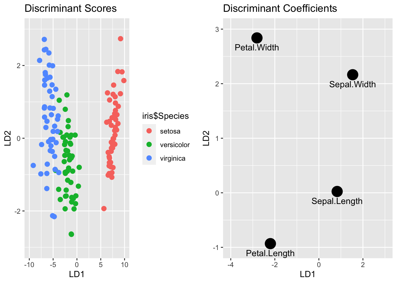

# visualize the LDA paritions
species <- factor(rep(c("s","c","v"), each=50))
partimat(x=dscores[,2:1], grouping=species, method="lda")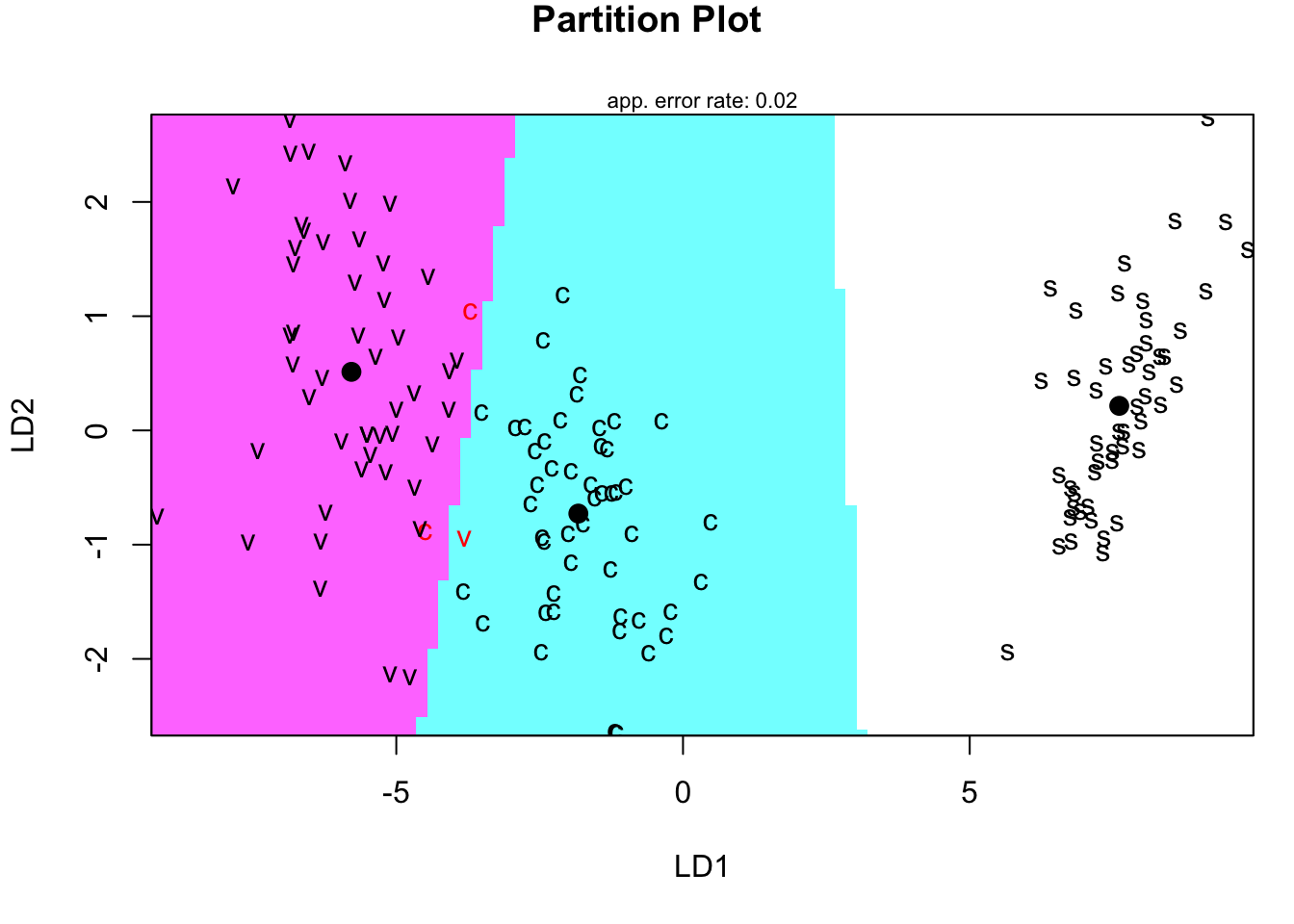

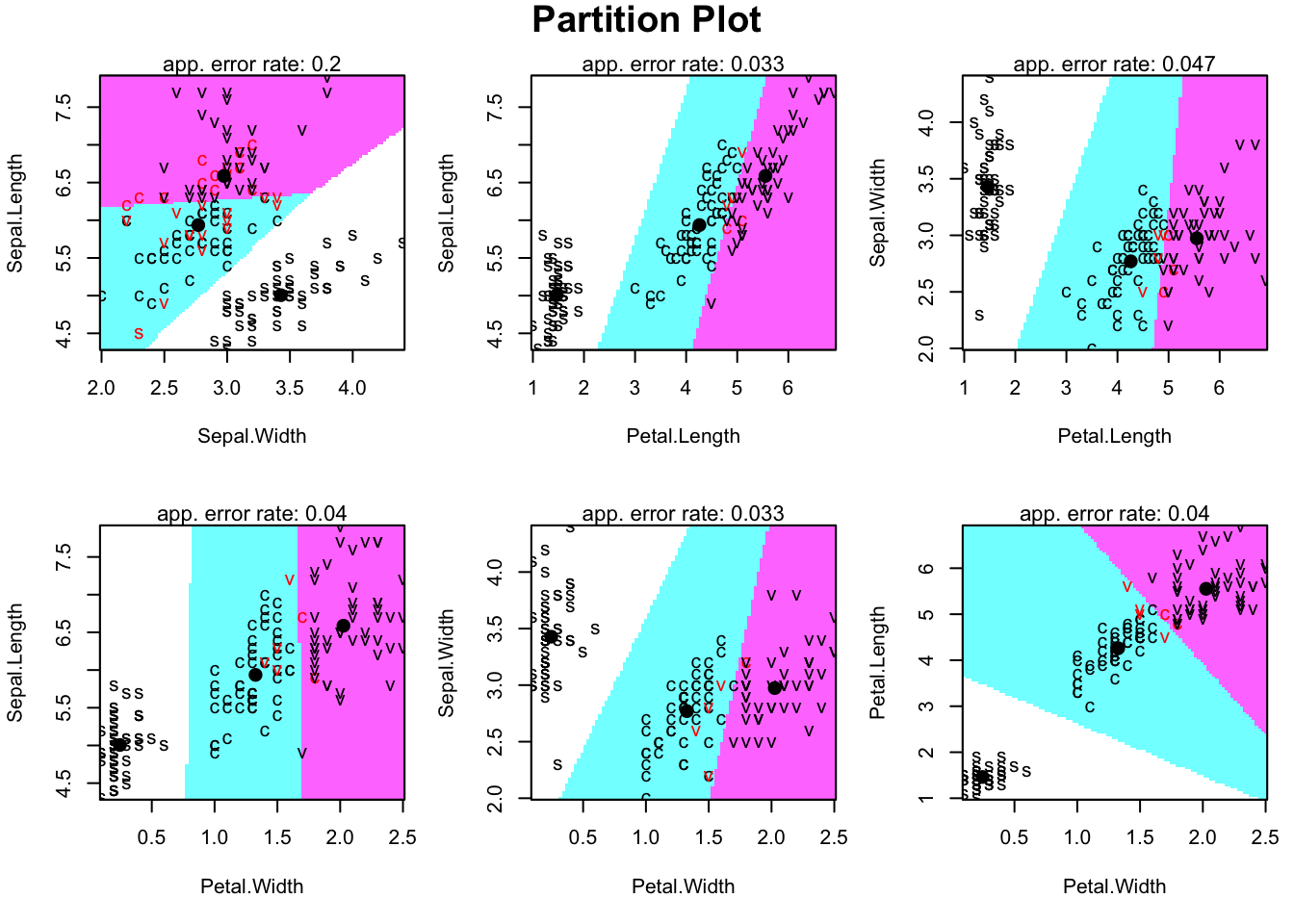
# visualize the LDA paritions (for all pairs)
species <- factor(rep(c("s","c","v"), each=50))
partimat(x=iris[,1:4], grouping=species, method="lda")