ONE-DIMENSIONAL ANALYSIS

We begin with exploratory data analysis, looking at variables separately in a one-dimensional way. This means we are only interested in empirical univariate distributions or parameters thereof, variable by variable, and do not yet analyze variables jointly or multivariately.

First we compute how often a specific value of a variable is observed. This is meaningful only when a variable has a finite set of possible values, that is, in technical terms, when the variable is measured on a discrete scale. Otherwise, if virtually any value of a variable is possible and each entry has a different value, the variable is measured on a continuous scale.

Now, consider we have as a starting point a sample with n observations for a variable \(X\) (e.g., thousands of observations for the variable \(FICO\) score in the mortgage database). For each observation we measure a specific value of the \(FICO\) score, denoted by \(x_1, ..., x_n\) , which is called the raw data. Let the variable be either discrete or continuous, but grouped into classes (e.g., \(FICO\) scores from \(350\) to \(370\), \(370\) to \(390\)). Then we denote the values or class numbers by \(a_1, ..., a_k\) and count the absolute numbers of occurrence of each value or class number by:

\[h_j = h(a_j)\]

and the relative frequencies by:

\[f_j = \frac{h_j}{n}\]

Moreover, we define the absolute and relative cumulative frequency \(H(x)\) and \(F(x)\) for each value \(x\) as the number or relative frequency of values being at most equal to \(x\) (i.e., being equal to \(x\) or lower). Graphically, this is a (nondecreasing) “stairway” function.

data <- read_csv('mortgage.zip')

## ! Multiple files in zip: reading ''mortgage.csv''

## 
## ── Column specification ────────────────────────────────────────────────────────
## cols(
##   .default = col_double()
## )
## ℹ Use `spec()` for the full column specifications.

attach(data)
freq(default_time, cum = T, total = T)

##            n     %  val%  %cum val%cum
## 0     607331  97.6  97.6  97.6    97.6
## 1      15158   2.4   2.4 100.0   100.0
## Total 622489 100.0 100.0 100.0   100.0

Next, we compute histograms, which plot the absolute (or relative) frequencies for values or classes of variables and the empirical cumulative distribution function (CDF) for the variable’s FICO score (FICO_orig_time) and LTV at origination (LTV_orig_time).

par(mfrow = c(2,2))
hist(FICO_orig_time, xlab = 'FICO')
plot(ecdf(FICO_orig_time), xlab = 'FICO')
hist(LTV_orig_time, xlab = 'LTV')
plot(ecdf(LTV_orig_time), xlab = 'LTV')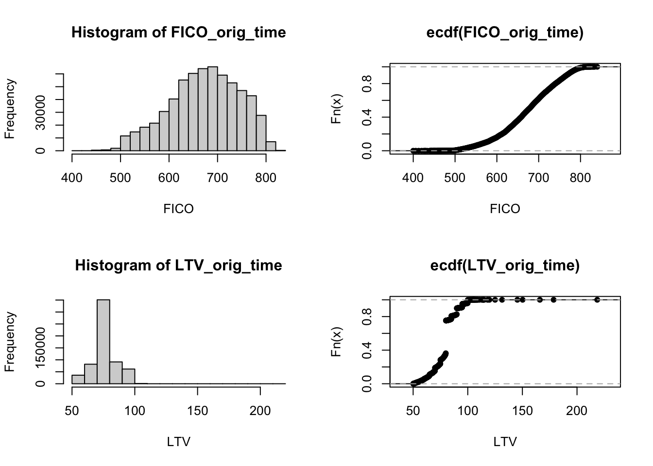

In addition, or as an alternative to the description of the entire distribution, we often report summarizing measures. These measures give numerical characterizations about the location of the distribution, its dispersion, and its shape, and are generally called moments.

summary(data.frame(default_time, FICO_orig_time, LTV_orig_time))

##   default_time     FICO_orig_time  LTV_orig_time   
##  Min.   :0.00000   Min.   :400.0   Min.   : 50.10  
##  1st Qu.:0.00000   1st Qu.:626.0   1st Qu.: 75.00  
##  Median :0.00000   Median :678.0   Median : 80.00  
##  Mean   :0.02435   Mean   :673.6   Mean   : 78.98  
##  3rd Qu.:0.00000   3rd Qu.:729.0   3rd Qu.: 80.00  
##  Max.   :1.00000   Max.   :840.0   Max.   :218.50

Quantiles can be used for a graphical comparison with standard distributions, such as a normal distribution. The normal distribution is widely used in applications and is a symmetric distribution with a single mode.

par(mfrow = c(1,2))
qqnorm(FICO_orig_time, pch = 1, frame = FALSE)
qqline(FICO_orig_time, col = "steelblue", lwd = 2)
qqnorm(LTV_orig_time, pch = 1, frame = FALSE)
qqline(LTV_orig_time, col = "darkred", lwd = 2)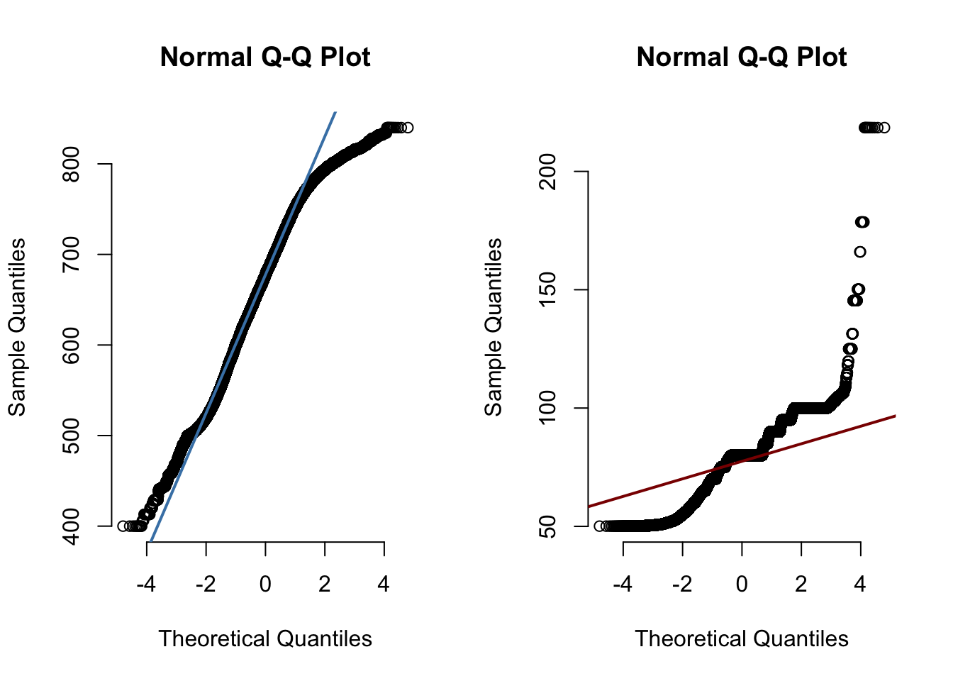

Next, we discuss the most commonly used dispersion measures and ones for the shape of the distribution, i.e. skewness and kurtosis.

psych::describe(data.frame(default_time, FICO_orig_time, LTV_orig_time))

##                vars      n   mean    sd median trimmed   mad   min   max range
## default_time      1 622489   0.02  0.15      0    0.00  0.00   0.0   1.0   1.0
## FICO_orig_time    2 622489 673.62 71.72    678  676.59 75.61 400.0 840.0 440.0
## LTV_orig_time     3 622489  78.98 10.13     80   79.21  7.41  50.1 218.5 168.4
##                 skew kurtosis   se
## default_time    6.17    36.09 0.00
## FICO_orig_time -0.32    -0.47 0.09
## LTV_orig_time  -0.20     1.44 0.01

TWO-DIMENSIONAL ANALYSIS

Having explored the empirical data on a one-dimensional basis for each variable, we are usually also interested in interrelations between variables; for example, if and how variables have a tendency to comove together. Thus, variables can be analyzed jointly and the joint empirical distribution can be examined. Moreover, summarizing measures for dependencies and comovements can be computed.

FICOrank <- cut(data$FICO_orig_time, seq(min(FICO_orig_time),max(FICO_orig_time),(max(FICO_orig_time)-min(FICO_orig_time))/5))
table(default_time, FICOrank)

##             FICOrank
## default_time (400,488] (488,576] (576,664] (664,752] (752,840]
##            0      1531     61138    199046    250160     95446
##            1        80      2222      6492      5426       938

prop.table(table(default_time, FICOrank))

##             FICOrank
## default_time    (400,488]    (488,576]    (576,664]    (664,752]    (752,840]
##            0 0.0024595207 0.0982169680 0.3197633976 0.4018770111 0.1533320803
##            1 0.0001285184 0.0035695983 0.0104292675 0.0087167599 0.0015068781

\(1531\) loans (or \(0.25\) percent of a total of \(n = 622489\) observations) had default status \(0\) and were in the lowest group (group \((400,488]\)) of the \(FICO\) scores. Altogether \(607321\) loans were not in default, which is \(97.56\) percent of all loans. Altogether, \(1611\) loans were in \(FICO\) group \((400,488]\). An important result we can infer from the table is that the proportion of loans that defaulted decreases the higher the \(FICO\) group becomes (from \(0.012\) percent in group \((400,488]\) to \(0.15\) percent in group \((752,840]\)). This leads to the conclusion that there should be some interrelation between FICO and default (i.e., the higher the FICO score, the lower the relative frequency of default).

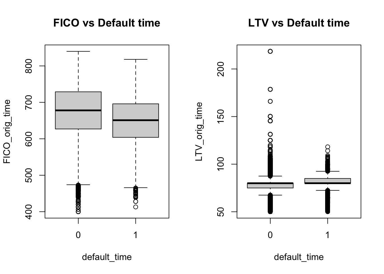
Another way of inferring the relation between both variables (without grouping FICO first) is to look at box plots. The location of the box is higher for FICO and lower for LTV in the nondefault category compared to the default category, which again shows some interrelation between the variables in the sense that higher FICO scores correspond to a lower default frequency and higher LTVs correspond to a higher default frequency.

default_time = as.factor(default_time)
par(mfrow = c(1,2))
boxplot(FICO_orig_time~default_time, main = 'FICO vs Default time')
boxplot(LTV_orig_time~default_time, main = 'LTV vs Default time')